This note covers implementing a raindrop and water flow effect on screen using URP's built-in Shader Graph. It also includes some commonly used Shader techniques. The overall approach can be divided into drawing raindrops, drawing trails, and blurring other parts.
Understanding UV
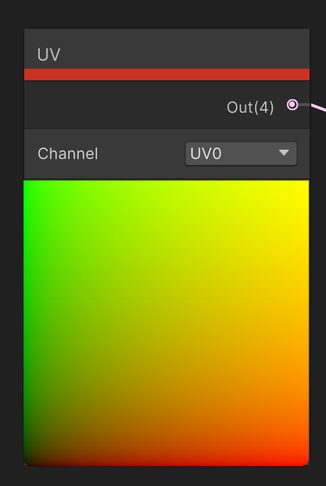
First, in Shader Graph, if we use the UV node directly to get UV coordinates, we see a preview like this:
Using the Swizzle node with Mask, we can inspect the x, y, z, w components.
In the preview, we know that 0 corresponds to darker colors and 1 to lighter colors. With homogeneous coordinates, we know the w component of a point is always 1, so the fourth texture is pure white. UV coordinates are 2D, so z is always 0. Focus on the x and y components, i.e., u and v. x goes from 0 to 1 left to right, and y goes from 0 to 1 bottom to top.
When we use Mask to extract the x and y values, we get this red-green color map.
Drawing Raindrops
Step 1: Draw a Circle
Drawing raindrops essentially means drawing a circle and showing the refraction of surrounding pixels inside it.
So the first step is to draw a circle. We can think of a circle as having constant distance from the center, so we need something related to center and distance. Simply put, it's the distance from a point on the UV to the origin—we can compute this with dot product and square root.
The effect of dot product + square root is identical to the Length node. From the figure above, we can see that the closer to the origin, the darker. We want to make the transition at the edge sharper. But we don't need to use distance from (0,0); for a circle-like shape, it's better to use distance from (0.5, 0.5).
Next, make the circle sharper. We want a smooth transition between min and max, with the range between them very tight so the edge becomes clear. The Smoothstep node does exactly this.
Connect the input to In, and map the distance output to between 0.11 and 0.1 to get a clear circle.
Step 2: Draw Many Circles
One circle isn't enough for raindrops—we want many. Suppose our UV range is [0,1] and we want to divide it into several segments. Let's try multiplying directly by the number of segments.
If RainSize is set to 4, the UV range goes from [0,1] to [0,4]. Values above 1 are displayed as yellow, so the Multiply result already has large yellow areas.
Is there a way to make each unit interval of length 1 display [0,1] colors? Yes—we ignore the integer part and only look at the fractional part. Use the Fraction node.
Very nice. We now have replicated UV colors; taking the distance from (0.5, 0.5) gives us multiple circles.
The raindrop circles shouldn't be too large. Adjust the circle size by changing the Smoothstep edge values.
[OPTIONAL] Step 2.5: Draw the UV Boundaries of Each Circle
For easier observation later, we can draw the UV boundaries of each circle. You can think about this yourself first, then compare with the node setup below.
Simply use the uv multiplied by RainSize with smoothstep to get the boundaries, then multiply by a color and add to the original circle map.
Step 3: Turn the Square Region into a Rectangle
Real raindrops typically move faster vertically and slower horizontally, so a rectangle works better than a square. This step is straightforward.
Change RainSize from a float to a 2D vector. But a new problem appears.
The circle becomes an ellipse. Fix this by dividing the value back.
Note: Because we divided by 2, the x UV range is now [0, 0.5], so when computing distance we should compare to (0.25, 0.5) instead of (0.5, 0.5).
Step 4: Move the Circles
Now make the circles move over time. First use the Time node. Simply add the Time output to the uv y value—split x and y, add Time to y, then recombine with the old x and new y.
After this, the circles should move vertically. But the motion is too uniform; add some variation. We want periodic variation, so use the sin function—subtract a time-varying sin value from y.
After this setup, you might see a circle moving oddly within its box, sometimes staying inside and sometimes going out. The speed is less uniform, but going out of bounds and overly regular motion are still not ideal.
Multiply sin by 0.3 to keep the circle within bounds. Then consider the movement period.
Use any graphing calculator. This is the graph of y = sin x. We want the periodic axis to shift to one side while keeping a clear periodicity.
Observe the graph of y = sin(x + sin(x + 0.5 sin(x))).
This basically meets our needs, so we'll use this function.
Create a new SubGraph and output this function's result.
Then use this function in the original SubGraph.
Drawing the Trail
The raindrop circles are mostly done. Now for the trail.
In the x direction, we don't need extra work. Assume the trail is multiple small water droplets following the large one. So we need to add a new UV range in the y direction, similar to the rectangle. Simply Multiply by a value.
Similarly, compute distance to the uv center and add a smoothstep (here we offset UV first then use Length; Length can be understood as distance from the origin). As before, remember to divide by the scale when recombining UV, or the raindrops may become elliptical.
Now there's a trail below the raindrop. We need to hide the trail below the raindrop.
Is there a node that returns the large circle's y value? Yes—the triple sin output above is the large circle's y. Apply smoothstep to this y so the lower half is black and the upper half white, then multiply by all the small circles.
Now the effect is that there are no small circles below the large circle.
Add a gradient to the non-time-varying y output above, then multiply by the existing circles for a fade effect.
X-Direction Oscillation
For oscillation in the x direction, use the sin function. The result should move within [0,1] in x, so use Subtract. The oscillation range must not exceed the border. (Use the second Multiply to control the sin output range.)
Then slightly adjust the scale on the sin composite function to ensure the shader runs as expected.
The x oscillation is currently independent of the y velocity, which we need to fix.
First, x oscillation should not be affected by time alone, so we should make sin independent of Time. From the curve analysis above, we can find a similar function related to sin(y). We won't elaborate here and will give a feasible setup directly. (You can also use a curve with similar speed variation.)
Now the trail follows this curve. That's still not right—we need to fix it.
Subtract them from time to make them relatively stationary.
Drawing the Path
Drawing the path left by the raindrop requires three parts: an image that is white above the raindrop and black below, another image that is white along the path and black on the sides, and a gradient from below the raindrop to the top of the UV region.
White Above, Black Below the Raindrop Boundary
This is simple—use Smoothstep.
Set edge1 and edge2 to -0.02 and 0 respectively.
White Along Path, Black on Sides
Use the X coordinate for the side boundaries, but remember to take the absolute value of X.
Multiply the two images above to get a map where only the path the raindrop has traveled has traces.
Gradient Map
Use the gradient map we made earlier.
You should now have this effect.