Realistic Water Simulation

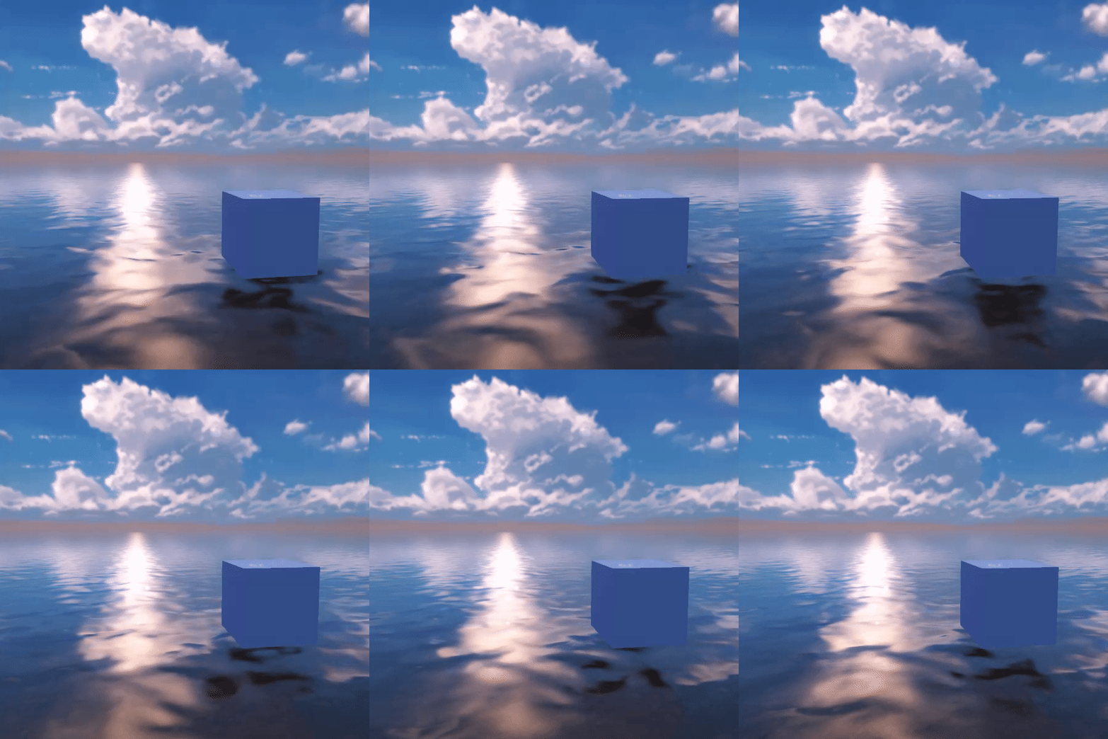
This project is a systematic study of realistic water simulation and rendering, written up as a paper for CMU's Visual Computing Systems course together with Moussab Ibrahim and Weier Flora Xiao. We implemented and compared the major families of real-time water techniques — from procedural wave superposition to FFT ocean spectra, and from particle-based fluids to Eulerian grid solvers — all GPU-accelerated with compute shaders in Unity.

The full paper is embedded at the bottom of this page; below is a tour of what it covers.

Surface Waves: From Oscillators to the FFT Ocean

Sum-of-sines and Gerstner waves

The simplest water surface is a height field driven by sine oscillators. A single sine wave looks unmistakably artificial, but superimposing waves with different frequencies, amplitudes, and directions already resembles a calm water surface:

$$h(\mathbf{x}, t) = \sum_i A_i \sin\big((\mathbf{k}_i \cdot \mathbf{x}) - \omega_i t + \varphi_i\big)$$

Real waves, though, have sharp crests and wide troughs that pure sine sums cannot produce. Gerstner waves fix this by displacing vertices horizontally as well as vertically, so points bunch up at crests — the classic trochoidal profile used in ocean shading ever since.

Statistical ocean modeling with the Phillips spectrum

Any finite sum of periodic waves eventually reveals its tiling when viewed from above. Oceanographic research treats wave height as a random variable with statistical regularities instead. Following Tessendorf, we synthesize the wave height field in Fourier space: each wave vector $\mathbf{k}$ gets a complex amplitude drawn from Gaussian noise, shaped by the Phillips spectrum

$$P_h(\mathbf{k}) = A \, \frac{e^{-1/(kL)^2}}{k^4} \, |\hat{\mathbf{k}} \cdot \hat{\mathbf{w}}|^2, \qquad L = \frac{V^2}{g}$$

which encodes wind speed $V$ and wind direction $\hat{\mathbf{w}}$ — waves perpendicular to the wind are suppressed, and a Gaussian factor $e^{-k^2 l^2}$ tames the poorly-converging short-wavelength tail.

Time evolution comes from the dispersion relation $\omega^2(k) = gk$: deep-water waves of different wavelengths travel at different speeds, which is exactly what makes an ocean surface feel alive:

$$\tilde{h}(\mathbf{k}, t) = \tilde{h}_0(\mathbf{k}) e^{i\omega(k)t} + \tilde{h}_0^*(-\mathbf{k}) e^{-i\omega(k)t}$$

The FFT that makes it real-time

Transforming the spectrum back to a spatial height field every frame requires an inverse DFT over a 512×512 grid — hopeless at $O(N^2)$, entirely practical at $O(N \log N)$. The paper walks through the Cooley-Tukey FFT from first principles: complex numbers as rotations, Euler's formula, the four-point butterfly operation, twiddle-factor symmetry, and how the divide-and-conquer stages assemble into the horizontal-then-vertical 1D FFT passes that produce the final height map on the GPU.

Volumetric Fluids: Particles and Grids

Height fields cannot splash. For genuinely three-dimensional behavior we implemented and compared three simulation families, all parallelized with Unity compute shaders.

Position-Based Fluids (PBF)

PBF sidesteps the stiffness problems of force-based SPH by working directly on positions: predict particle positions from velocity and gravity, then iteratively project them onto the incompressibility constraint

$$C_i = \frac{\rho_i}{\rho_0} - 1 = 0$$

where density $\rho_i$ is estimated with the poly6 smoothing kernel over neighbors, and corrections $\Delta \mathbf{p}_i$ are distributed via per-particle Lagrange multipliers. A uniform grid-based neighbor search (cell size = interaction radius, 27-cell lookup) brings the neighbor query from $O(n^2)$ down to effectively $O(n)$, which is what makes tens of thousands of particles interactive.

Smoothed Particle Hydrodynamics (SPH)

The classical force-based formulation of the Navier-Stokes momentum equation: pressure forces, viscosity forces, and density all evaluated through smoothing kernels (poly6 for density, spiky gradient for pressure, viscosity Laplacian). With GPU indirect instancing we reached ~10,000 particles in real time. SPH captures droplets and splashes beautifully but demands careful time-step and stiffness tuning — instructive pain that motivated the PBF implementation.

Eulerian grid solver

The opposite worldview: fix the space, not the particles. Velocity and density live on a staggered grid; each step performs semi-Lagrangian advection, then enforces $\nabla \cdot \mathbf{v} = 0$ with a Gauss-Seidel pressure projection. Parallelizing Gauss-Seidel on a GPU is non-trivial because neighboring cells share edges — we used a checkerboard partition that splits cells into two disjoint groups so each half-grid updates concurrently without race conditions. The grid method proved markedly more stable than SPH and scaled past 10,000 cells.

Screen-Space Fluid Rendering

Particles are not a surface. To shade the PBF simulation as continuous water we implemented the screen-space fluid rendering pipeline:

1. Particle spheres — expand each particle into a camera-facing quad in the geometry shader, discard pixels outside the sphere.
2. Depth pass — render particle depth, encoded for later passes.
3. Bilateral blur — smooth the depth buffer while preserving silhouettes, melting individual particles into a coherent surface.
4. Normal reconstruction — rebuild eye-space normals from depth gradients via cross products.
5. Thickness pass — additive blending without depth test measures how much fluid each ray traverses.
6. Shading — diffuse + ambient + specular, volumetric absorption via Beer-Lambert attenuation $I = e^{-kd}$, and Fresnel reflectance through the Schlick approximation.

The result reads as a transparent, refractive liquid volume — computed entirely from particle data, with no meshing step.

What This Project Demonstrates

• Breadth across the water stack — procedural waves, spectral ocean synthesis, three fluid simulation paradigms, and a complete screen-space rendering pipeline, implemented rather than surveyed.
• The math behind the effects — complex analysis and the FFT derived from scratch; spectra, dispersion, and smoothing kernels applied with an understanding of where each breaks down.
• GPU engineering judgment — compute-shader parallelization, race-condition-free Gauss-Seidel, grid-based neighbor acceleration, and honest trade-off analysis between SPH, PBF, and Eulerian methods (stability vs. detail vs. scalability).

The full 13-page paper:

Realistic Water Simulation — Full PaperOpen ↗